Video Coding History
Sending visual images to a remote location has captured the human imagination for more than a century (Figure 1). The invention of television in 1926 by the Scotsman John Logie Baird led to the realisation of this concept over analogue communication channels. Even analogue TV systems made use of compression or information reduction to fit higher resolution visual images into limited transmission bandwidths.
Figure 1 - "in the year 2000", postcard from 1910
The emergence of mass market digital video in the 1990s was made possible by compression techniques that had been developed during the preceding decades. Even though the earliest videophones and consumer digital video formats were limited to very low resolution images (352x288 pixels or smaller), the amount of information required to store and transmit moving video was too great for the available transmission channels and storage media. Video coding or compression was an integral part of these early digital applications and it has remained central to each further development in video technology since 1990.
By the early 1990s, many of the key concepts required for efficient video compression had been developed. During the 1970s, industry experts recognised that video compression had the potential to revolutionise the television industry. Efficient compression would make it possible to transmit many more digital channels in the bandwidth occupied by the older analogue TV channels.
Present-day video coding standards and products share the following features:
Motion compensated prediction from one or more previously encoded frames or fields.
Subtraction of a motion compensated prediction from the current basic unit, to form a residual unit (e.g. a residual MB).
Block transform and quantization to form blocks of quantized coefficients.
Entropy encoding of quantized coefficients and side information such as motion vectors and headers
1. Entropy coding
David Huffman’s paper on Minimum Redundancy Codes, published in 1952 [1], described a method of constructing codewords with multiple digits to efficiently encode a message with a finite alphabet of symbols. This is the basis of the well- known Huffman Coding method, which represents symbols by variable length, uniquely decodable binary codewords. Versions of Huffman Coding were used in early video coding standards including H.261, H.263, MPEG-1, MPEG-2 and MPEG-4 Part 2.
Rissanen’s 1976 paper on Arithmetic Coding [2] was extended by Witten in 1987 [3] to provide a practical alternative to Huffman variable length coding. The strength of Arithmetic Coding is that symbols do not have to be represented with an exact integral number of bits, making it possible to out-perform variable length coding with integral bit counts per codeword.
2. Frame differencing
The aim of prediction in a video codec is to:
Generate a prediction of the information to be coded, based on previously processed data and
Subtract this prediction from the information to be coded.
The more accurate the prediction, the less information remains after step 2.
An early contribution to this concept was a patent by B M Oliver, published in 1956 [4]. Oliver’s patent was specifically directed towards reducing the channel capacity required to transmit signals such as television signals: “It is a primary object of the present invention to increase the efficiency of transmission systems now commonly in use for the communication of intelligence by reducing the redundancy in the signals which are transmitted” – what we now describe as video compression.
Figure 3 of Oliver’s patent (Figure 2) bears a striking resemblance to the modern video codec model, with a predictor (44), a subtractor (41), a quantizer (42) and a reconstructor or adder (43). Oliver describes the general concepts of both spatial prediction and temporal prediction: “Often, the previous samples used to determine a particular predicted value will comprise primarily immediately preceding samples”… [i.e. spatial prediction], “but in certain cases, such as in a television signal… there may be more advantageously be utilized samples a considerable number of sampling intervals previous in time” [i.e. temporal prediction].
Figure 2 - Figure from Oliver, 1956, showing prediction and quantization
Oliver’s work was primarily directed towards data compression for transmission of analogue signals such as television. Manfred Schroeder of Bell Labs applied the prediction concept specifically to video signals “preferably… in digital form” in his 1972 patent [5]. Schroeder’s model (Figure 3) introduces a transform coder (12) to “distribute” the difference or error signal “over the entire frame”, so as to provide a relatively constant information content to the quantizer 13. Schroeder’s 1972 patent provides an early disclosure of frame differencing, transform coding and quantization. There is no mention of motion compensated prediction or of entropy coding. A number of publications in the early 1970s investigated different aspects of frame differencing and conditional replenishment [6,7].
Figure 3 - Figure from Schroeder, 1972, showing frame differencing and transform coding
3. The Discrete Cosine Transform
In their classic 1974 paper, Ahmed, Natarajan and Rao introduced a new transform for image processing, the Discrete Cosine Transform [8]. The authors explained its potential benefits in applications such as pattern recognition and Wiener filtering.
The DCT closely approximates the performance of the theoretically ideal Karhunen-Loeve Transform KLT but has the significant advantage of being relatively easy to compute (Figure 4).
Chen, Smith and Fralick described a fast, low complexity implementation of the DCT in 1977 [9], making it an attractive choice for practical image and video codecs, in terms of compression performance and computational efficiency. The DCT was to become the transform of choice for video codecs from the 1980s onwards.
Figure 4 - Basis patterns of the 8x8 DCT
4. Motion compensated interframe coding
Netravali and Stuller [10] introduce the concept of motion compensated prediction in their 1979 paper. The first encoding step is a DCT, followed by prediction in the transform domain. Two motion compensated prediction techniques are described. In the first, estimates of displacement are transmitted to the decoder. In the second, displacement estimates are calculated from previously transmitted transform coefficients, so that the estimates need not be transmitted.
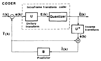
In their 1981 paper, Jain and Jain [11] describe a codec that is close to the modern- day model (Figure 5). Motion compensated prediction is carried out in the transform domain, after a 2-dimensional DCT is applied to each block. A search unit finds the optimal displacement vector (motion vector) which is transmitted along with the prediction residual.
Figure 5 - Motion compensated interframe coder, Jain and Jain, 1981
By 1985, all of the main elements were being brought together. Staffan Ericsson [12] describes a coder (Figure 6) that incorporates:
Motion compensated prediction of rectangular blocks, using sub-pixel interpolation
16x16 DCT
Quantization of DCT coefficients
Diagonal (zig-zag) scanning of quantized coefficients
Run-level and Huffman coding
Bit rate control by modifying the quantizer step size.
The basic codec model was now complete and was to be used again and again, with successive refinements of each component, in the video coding standards of the 1990s and 2000s.
Figure 6 - Video encoder, Staffan Ericson, 1985
About Vcodex
Vcodex helps companies realize the full value of their video technology. We provide world-class expertise in:
Video and image compression coding
Video streaming and transmission
Multimedia processing architectures
Visual quality analysis.
Vcodex is led by Iain Richardson, an international expert in video compression. The author of four widely cited books on video coding, Professor Richardson is an experienced expert witness who advises companies worldwide on video compression technology, video coding patents and technology acquisitions.
References
1 “A Method for the Construction of Minimum Redundancy Codes”, D A Huffman, Proceedings of the I.R.E., September 1952.
2 “Generalized Kraft inequality and arithmetic coding”, J J Rissanen, IBM J. Res. Dev. 20, May 1976.
3 “Arithmetic coding for data compression”, I Witten, R Neal and J Cleary, Communications of the ACM, June 187.
4 “Linear predictor circuits”, B M Oliver, US Patent 2732424, 1956.
5 “Transform coding of image difference signals”, M R Schroeder, US Patent 3679821, 1972.
6 “Interframe coding of videotelephone pictures”, Haskell, Mounts and Candy, Proc. IEEE, July 1972.
7 “A video encoding system using conditional picture element replenishment”, F W Mounts, Bell System Technical Journal, September 1969.
8 “Discrete Cosine Transform”, Ahmed, Natarajan and Rao, IEEE Transactions on Computers, Jan 1974.
9 “A fast computational algorithm for the Discrete Cosine Transform”, Chen, Smith and Fralick, IEEE Trans. Communications, September 1977.
10 “Motion compensated transform coding”, A N Netravali and J A Stuller, Bell System Technical Journal, September 1979.
11 “Displacement measurement and its application to interframe image coding”, J R Jain and A K Jain, IEEE Trans. Communications, December 1981.
12 “Fixed and adaptive predictors for hybrid predictive / transform coding”, Staffan Ericsson, IEEE Trans. Communications, December 1985.